3  Tutorial 3: Deep neural network with explainable method (binary classification)

Aims: To predict heart disease using a deep neural network - To explain model predictions using Layer-wise Relevance Propagation (LRP) - To visualize feature importance at both individual and global levels

Data: heartdisease data from MLDataR package.

Code description: This code demonstrates the use of torch with custom dataset functions, training callbacks, and model explainability using the innsight package for binary classification with LRP.

Packages

library(torch)
library(luz)
library(tidyverse)
library(tidymodels)
library(MLDataR)
library(innsight)

Data

heart_df <- 
  heartdisease %>% 
  mutate(across(c(Sex, RestingECG, Angina), as.factor))

Explore data.

skimr::skim(heart_df)

Data summary

Name	heart_df
Number of rows	918
Number of columns	10
_______________________
Column type frequency:
factor	3
numeric	7
________________________
Group variables	None

Variable type: factor

skim_variable	n_missing	complete_rate	ordered	n_unique	top_counts
Sex	0	1	FALSE	2	M: 725, F: 193
RestingECG	0	1	FALSE	3	Nor: 552, LVH: 188, ST: 178
Angina	0	1	FALSE	2	N: 547, Y: 371

Variable type: numeric

skim_variable	n_missing	complete_rate	mean	sd	p0	p25	p50	p75	p100	hist
Age	0	1	53.51	9.43	28.0	47.00	54.0	60.0	77.0	▁▅▇▆▁
RestingBP	0	1	132.40	18.51	0.0	120.00	130.0	140.0	200.0	▁▁▃▇▁
Cholesterol	0	1	198.80	109.38	0.0	173.25	223.0	267.0	603.0	▃▇▇▁▁
FastingBS	0	1	0.23	0.42	0.0	0.00	0.0	0.0	1.0	▇▁▁▁▂
MaxHR	0	1	136.81	25.46	60.0	120.00	138.0	156.0	202.0	▁▃▇▆▂
HeartPeakReading	0	1	0.89	1.07	-2.6	0.00	0.6	1.5	6.2	▁▇▆▁▁
HeartDisease	0	1	0.55	0.50	0.0	0.00	1.0	1.0	1.0	▆▁▁▁▇

Dataset function

heart_dataset <- dataset(
  initialize = function(df) {
    # Pre-process and store as tensors
    self$x_num <- df %>% 
      select(Age, RestingBP, Cholesterol, FastingBS, MaxHR, HeartPeakReading) %>% 
      mutate(across(everything(), scale)) %>% 
      as.matrix() %>% 
      torch_tensor(dtype = torch_float())
    
    self$x_cat <- model.matrix(~ Sex + RestingECG + Angina, data = df)[, -1] %>% 
      as.matrix() %>% 
      torch_tensor(dtype = torch_float())
    
    self$y <- torch_tensor(as.matrix(df$HeartDisease), dtype = torch_float())
  },
  .getitem = function(i) {
    list(x = list(self$x_num[i, ], self$x_cat[i, ]), y = self$y[i])      
  },
  .length = function() {
    self$y$size(1)
  }
)

# Convert to torch dataset
ds_tensor <- heart_dataset(heart_df)
ds_tensor[1]

$x
$x[[1]]
torch_tensor
-1.4324
 0.4107
 0.8246
-0.5510
 1.3822
-0.8320
[ CPUFloatType{6} ]

$x[[2]]
torch_tensor
 1
 1
 0
 0
[ CPUFloatType{4} ]


$y
torch_tensor
 0
[ CPUFloatType{1} ]

Split data with dataset subsets

set.seed(123) 
n <- nrow(heart_df)
train_size <- floor(0.6 * n)
valid_size <- floor(0.2 * n)

# Create indices
all_indices <- 1:n
train_indices <- sample(all_indices, size = train_size)

remaining_indices <- setdiff(all_indices, train_indices)
valid_indices <- sample(remaining_indices, size = valid_size)

test_indices <- setdiff(remaining_indices, valid_indices)

# Create Subsets
train_ds <- dataset_subset(ds_tensor, train_indices)
valid_ds <- dataset_subset(ds_tensor, valid_indices)
test_ds  <- dataset_subset(ds_tensor, test_indices)

Convert to dataloader

train_dl <- train_ds %>% 
  dataloader(batch_size = 10, shuffle = TRUE)

valid_dl <- valid_ds %>% 
  dataloader(batch_size = 10, shuffle = FALSE)

test_dl <- test_ds %>% 
  dataloader(batch_size = 10, shuffle = FALSE)

Specify the model

net <- 
  nn_module(
    initialize = function(d_in){
      self$net <- nn_sequential(
        nn_linear(d_in, 32),
        nn_relu(),
        nn_dropout(0.5),
        nn_linear(32, 64),
        nn_relu(),
        nn_dropout(0.5),
        nn_linear(64, 1),
        nn_sigmoid()
      )
    },
    forward = function(x){
      # x is currently a list of two tensors (numeric and categorical)
      # Concatenate them along the feature dimension (dim=2)
      input <- torch_cat(x, dim = 2)
      self$net(input)
    }
  )

Fit the model

Set parameters

d_in <- length(ds_tensor[1]$x[[1]]) + length(ds_tensor[1]$x[[2]]) # total number of features (6 numeric + 4 categorical = 10)

Fit with callbacks

fitted <- 
  net %>% 
  setup(
    loss = nn_bce_loss(),
    optimizer = optim_adam,
    metrics = list(
      luz_metric_binary_accuracy(), 
      luz_metric_binary_auroc()
    )
  ) %>% 
  set_hparams(d_in = d_in) %>% 
  fit(
    train_dl, 
    epoch = 50, 
    valid_data = valid_dl,
    callbacks = list(
      luz_callback_early_stopping(patience = 10),
      luz_callback_keep_best_model()
    )
  )

Training plot

fitted %>% plot()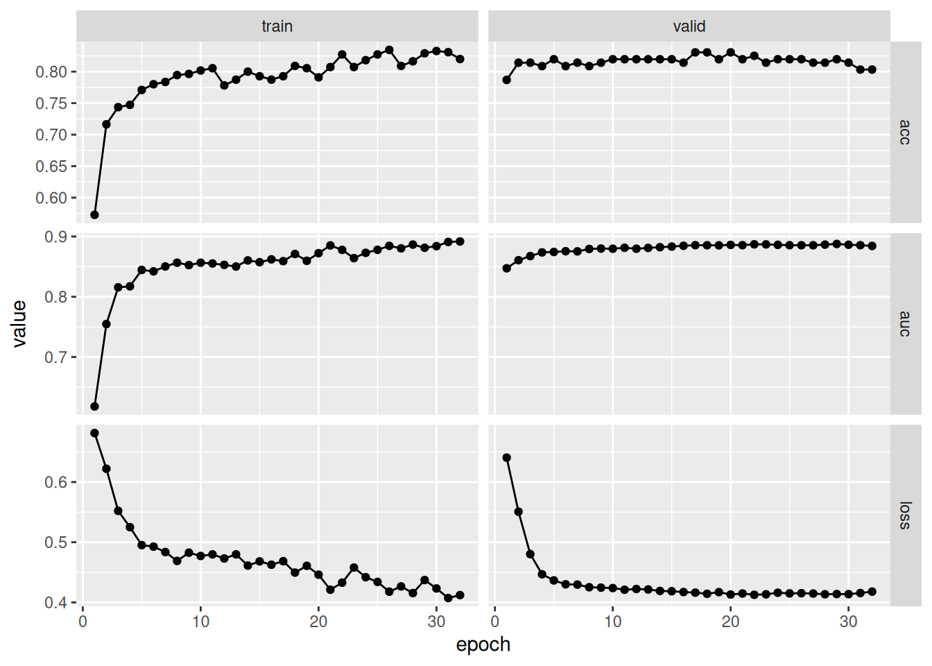

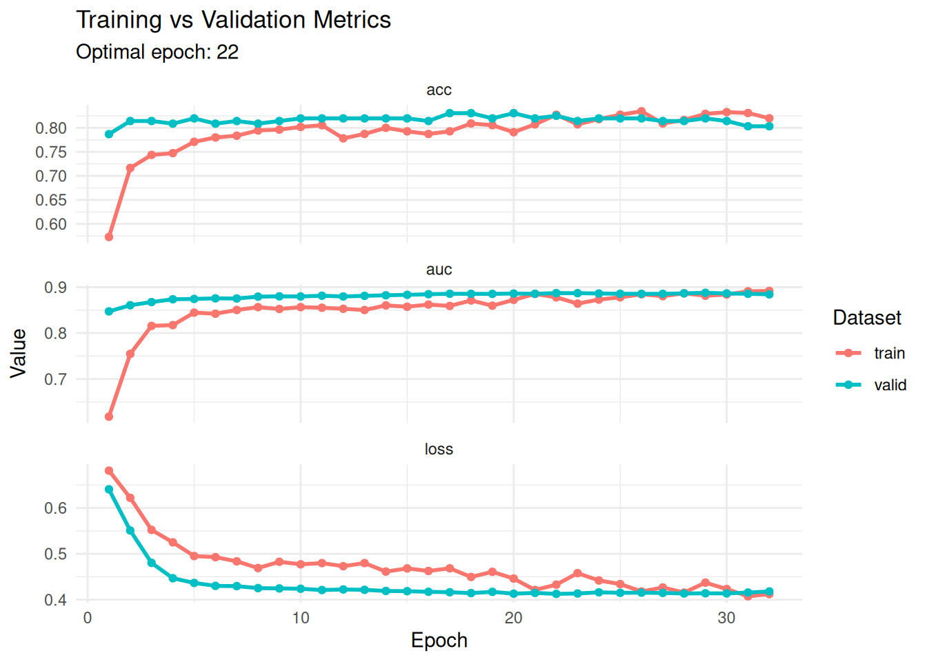
Better plot

hist <- get_metrics(fitted)

optimal_epoch <- hist %>%
  filter(metric == "loss", set == "valid") %>%
  slice_min(value, n = 1) %>%
  pull(epoch)

hist %>%
  ggplot(aes(x = epoch, y = value, color = set)) +
  geom_line(linewidth = 1) +
  geom_point(size = 1.5) +
  facet_wrap(~ metric, scales = "free_y", ncol = 1) +
  theme_minimal() +
  labs(
    title = "Training vs Validation Metrics",
    subtitle = paste("Optimal epoch:", optimal_epoch),
    y = "Value",
    x = "Epoch",
    color = "Dataset"
  )

Predict testing set

y_pred <- fitted %>% predict(test_dl)
y_true <- ds_tensor$y[test_ds$indices] %>% as_array()

dat_pred <- 
  y_pred %>% 
  as_array() %>% 
  as_data_frame() %>% 
  rename(prob = V1) %>% 
  mutate(
    pred = factor(ifelse(prob > 0.5, 1, 0)),
    true = factor(y_true)
  )

Warning: `as_data_frame()` was deprecated in tibble 2.0.0.
ℹ Please use `as_tibble()` (with slightly different semantics) to convert to a
  tibble, or `as.data.frame()` to convert to a data frame.

Warning: The `x` argument of `as_tibble.matrix()` must have unique column names if
`.name_repair` is omitted as of tibble 2.0.0.
ℹ Using compatibility `.name_repair`.
ℹ The deprecated feature was likely used in the tibble package.
  Please report the issue at <https://github.com/tidyverse/tibble/issues>.

dat_pred

# A tibble: 185 × 3
     prob pred  true 
    <dbl> <fct> <fct>
 1 0.0886 0     0    
 2 0.326  0     0    
 3 0.0819 0     0    
 4 0.957  1     1    
 5 0.0911 0     0    
 6 0.182  0     0    
 7 0.311  0     0    
 8 0.383  0     0    
 9 0.871  1     0    
10 0.102  0     1    
# ℹ 175 more rows

Evaluate

fitted %>% evaluate(test_dl)

A `luz_module_evaluation`
── Results ─────────────────────────────────────────────────────────────────────
loss: 0.4137
acc: 0.8216
auc: 0.8852

Confusion matrix

dat_pred %>% 
  conf_mat(true, pred) %>% 
  autoplot("heatmap")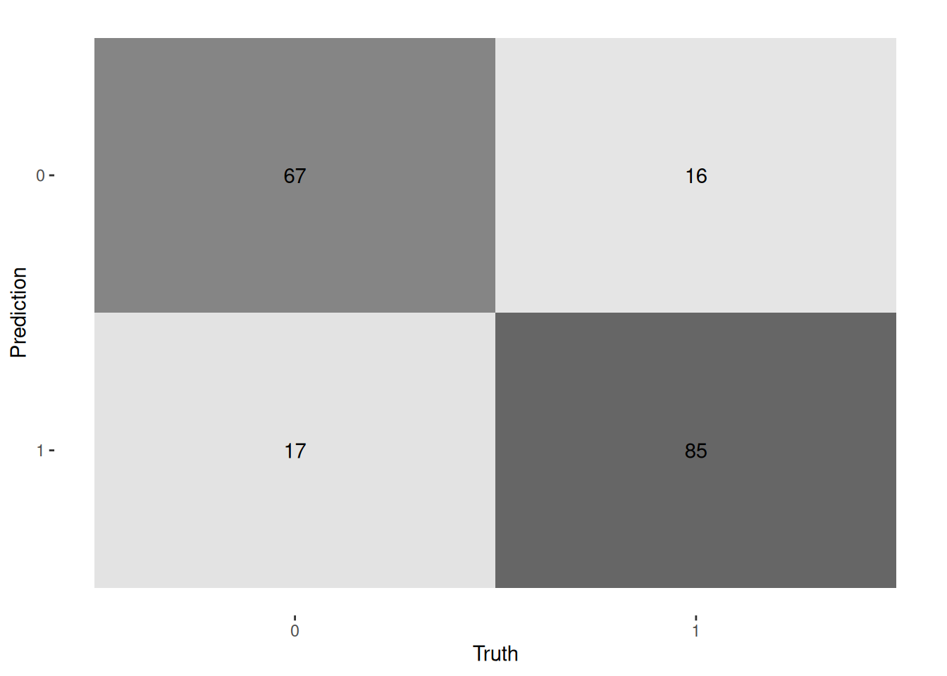

Accuracy

dat_pred %>% 
  accuracy(truth = true, estimate = pred)

# A tibble: 1 × 3
  .metric  .estimator .estimate
  <chr>    <chr>          <dbl>
1 accuracy binary         0.822

Plot ROC

dat_pred %>% 
  roc_curve(true, prob, event_level = "second") %>% 
  autoplot()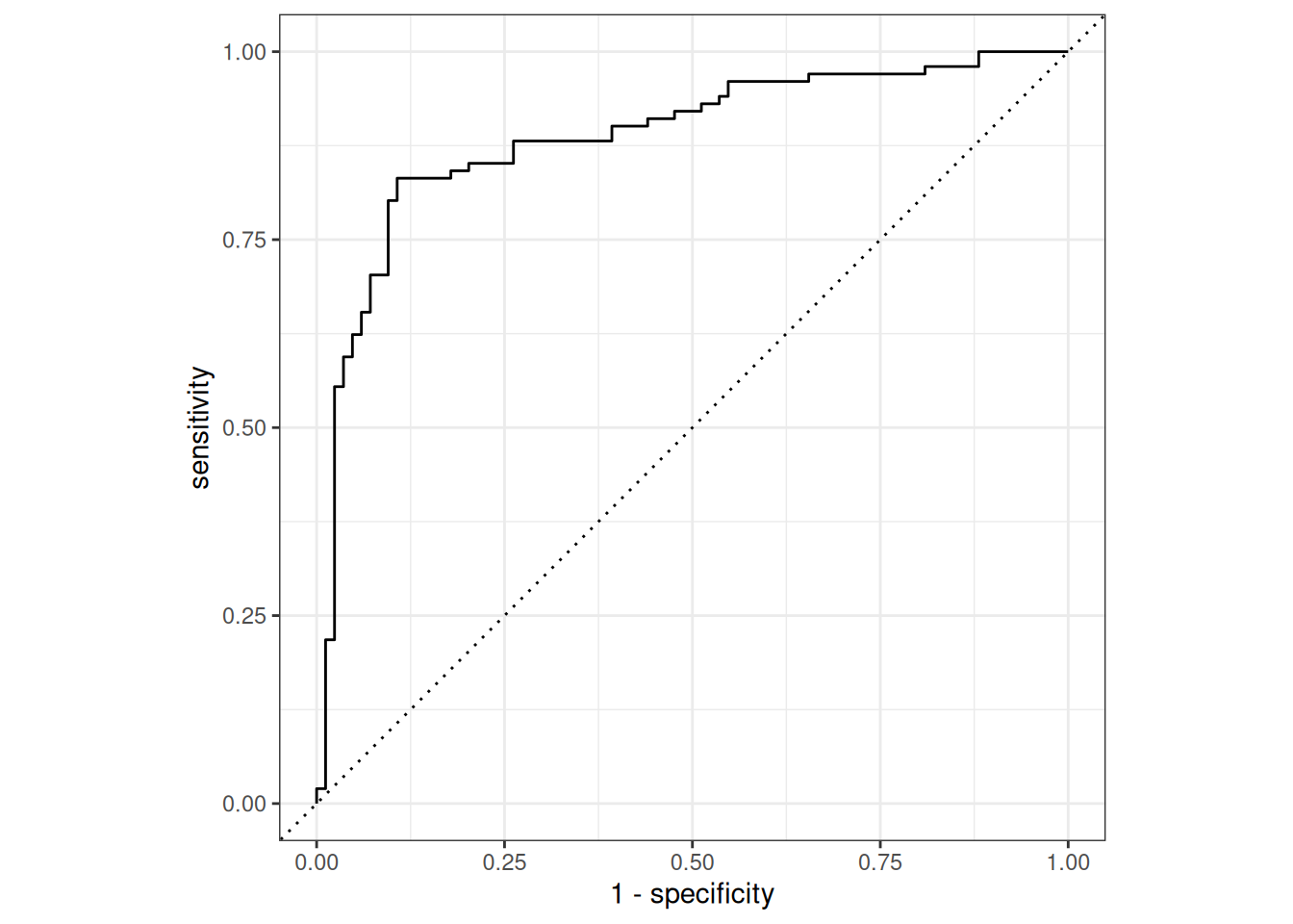

# ROC-AUC
dat_pred %>% 
  roc_auc(true, prob, event_level = "second")

# A tibble: 1 × 3
  .metric .estimator .estimate
  <chr>   <chr>          <dbl>
1 roc_auc binary         0.887

Model explainability with LRP

Prepare model for interpretation.

# Extract the sequential model
model <- fitted$model$net$cpu()

# Define input and output names
input_names <- c(
  # Numeric variables
  "Age", "RestingBP", "Cholesterol", "FastingBS", "MaxHR", "HeartPeakReading",
  # Categorical dummies (from model.matrix ~ .-1)
  "Sex_M", "RestingECG_Normal", "RestingECG_ST", "Angina_Y"
)

output_names <- c("Probability of heart disease")

Create converter and prepare test data.

# Create the Converter object
converter <- convert(
  model,
  input_dim = 10,
  input_names = input_names,
  output_names = output_names
)

Skipping nn_dropout ...
Skipping nn_dropout ...

# Manually extract and concatenate the test data
idxs <- test_ds$indices
x_num <- ds_tensor$x_num[idxs, ]
x_cat <- ds_tensor$x_cat[idxs, ]

# Combine into one tensor and convert to R array
input_tensor <- torch_cat(list(x_num, x_cat), dim = 2)
input_data <- as_array(input_tensor)

Apply Layer-wise Relevance Propagation (LRP).

# Run LRP with alpha-beta rule
lrp_result <- run_lrp(converter, input_data, rule_name = "alpha_beta", rule_param = 1)

# Check dimensions: Instances x Features x Outputs
dim(get_result(lrp_result))

[1] 185  10   1

Individual explanations.

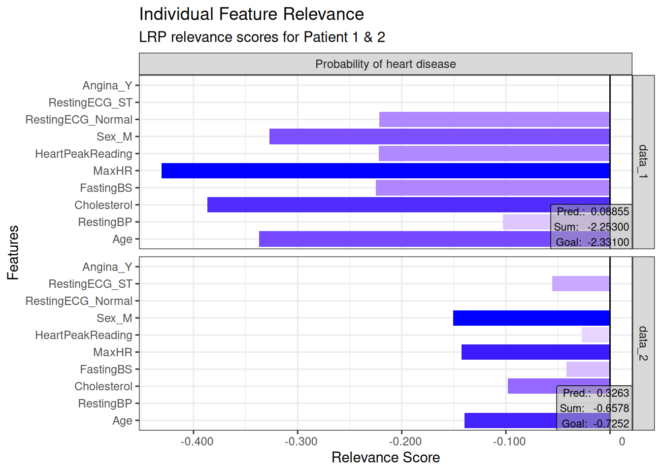
# Individual plots for the first two test instances
plot(lrp_result, data_idx = c(1, 2)) +
  theme_bw() +
  coord_flip() +
  labs(
    title = "Individual Feature Relevance",
    subtitle = "LRP relevance scores for Patient 1 & 2",
    x = "Features",
    y = "Relevance Score"
  )

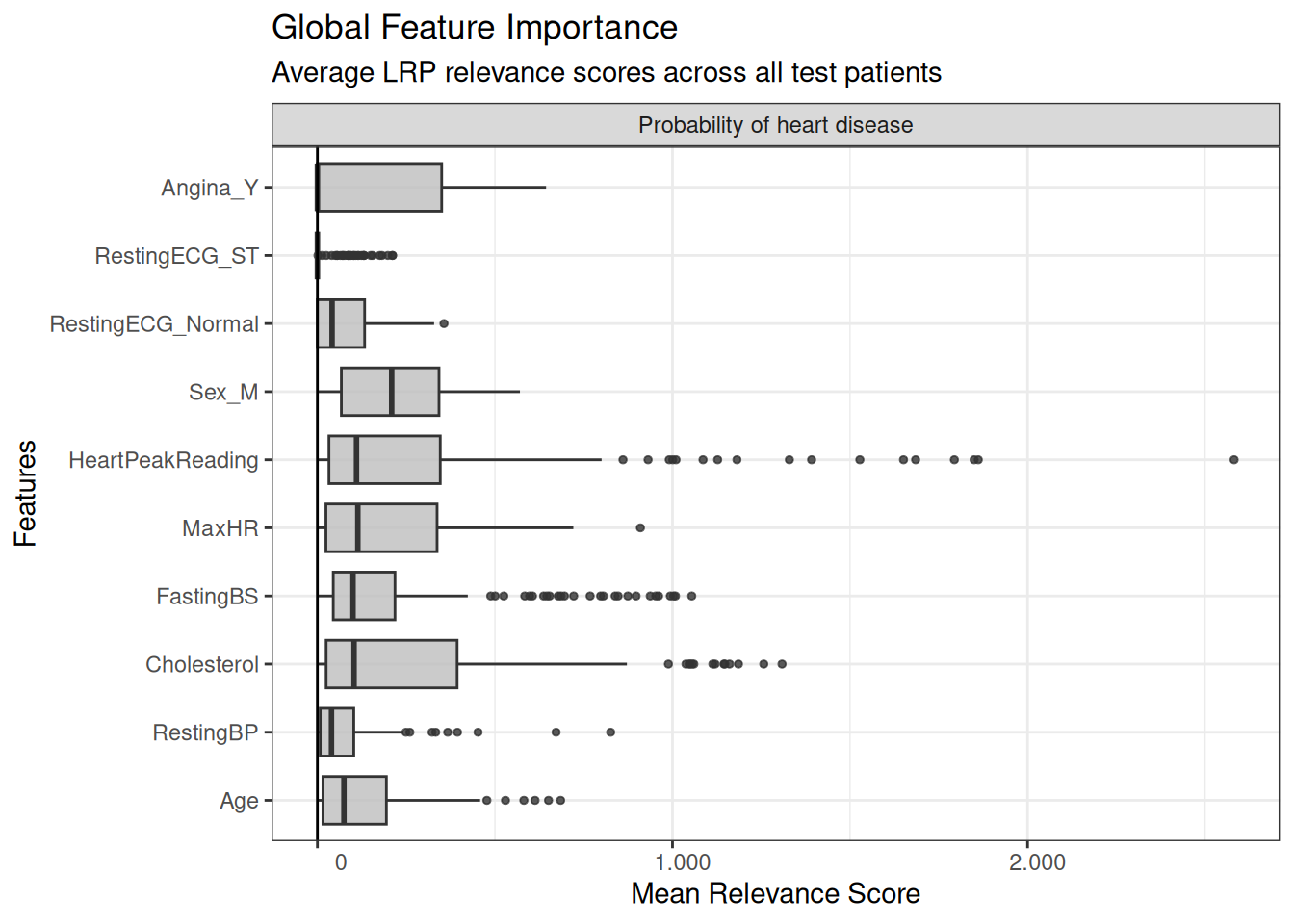
Global explanations.

# Global boxplot - overall feature importance across the entire test set
boxplot(lrp_result) +
  theme_bw() +
  coord_flip() +
  labs(
    title = "Global Feature Importance",
    subtitle = "Average LRP relevance scores across all test patients",
    x = "Features",
    y = "Mean Relevance Score"
  )

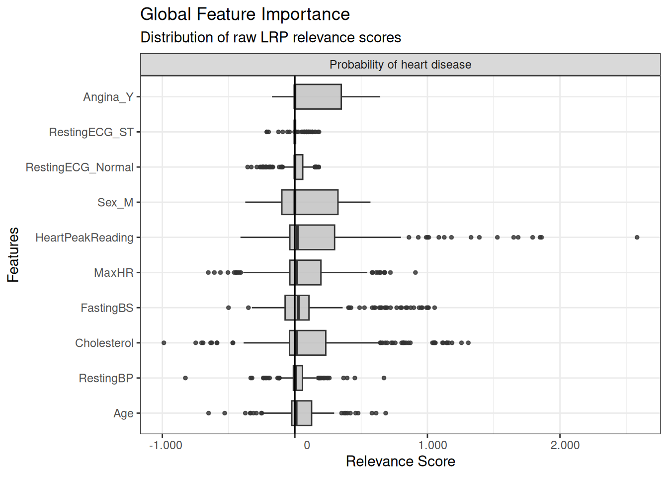
Global explanation with raw relevance scores.

# Another version of global boxplot with identity transformation
boxplot(lrp_result, preprocess_FUN = identity) +
  theme_bw() +
  coord_flip() +
  labs(
    title = "Global Feature Importance",
    subtitle = "Distribution of raw LRP relevance scores",
    x = "Features",
    y = "Relevance Score"
  )