library(torch)
library(luz)
library(tidyverse)
library(tidymodels)
library(MLDataR)1 Tutorial 1: Basic deep neural network (binary classification)
Aims: To predict a heart disease using a deep neural network.
Data: heartdisease data from MLDataR package.
Code description: This codes demonstrate the use of deep neural network through torch but at the same time, still using tidymodels functions for splitting data, preprocessing, and performance metrics.
Packages
Data
heart_df <-
heartdisease %>%
mutate(across(c(Sex, RestingECG, Angina), as.factor))
Explore data.
skimr::skim(heart_df)| Name | heart_df |
| Number of rows | 918 |
| Number of columns | 10 |
| _______________________ | |
| Column type frequency: | |
| factor | 3 |
| numeric | 7 |
| ________________________ | |
| Group variables | None |
Variable type: factor
| skim_variable | n_missing | complete_rate | ordered | n_unique | top_counts |
|---|---|---|---|---|---|
| Sex | 0 | 1 | FALSE | 2 | M: 725, F: 193 |
| RestingECG | 0 | 1 | FALSE | 3 | Nor: 552, LVH: 188, ST: 178 |
| Angina | 0 | 1 | FALSE | 2 | N: 547, Y: 371 |
Variable type: numeric
| skim_variable | n_missing | complete_rate | mean | sd | p0 | p25 | p50 | p75 | p100 | hist |
|---|---|---|---|---|---|---|---|---|---|---|
| Age | 0 | 1 | 53.51 | 9.43 | 28.0 | 47.00 | 54.0 | 60.0 | 77.0 | ▁▅▇▆▁ |
| RestingBP | 0 | 1 | 132.40 | 18.51 | 0.0 | 120.00 | 130.0 | 140.0 | 200.0 | ▁▁▃▇▁ |
| Cholesterol | 0 | 1 | 198.80 | 109.38 | 0.0 | 173.25 | 223.0 | 267.0 | 603.0 | ▃▇▇▁▁ |
| FastingBS | 0 | 1 | 0.23 | 0.42 | 0.0 | 0.00 | 0.0 | 0.0 | 1.0 | ▇▁▁▁▂ |
| MaxHR | 0 | 1 | 136.81 | 25.46 | 60.0 | 120.00 | 138.0 | 156.0 | 202.0 | ▁▃▇▆▂ |
| HeartPeakReading | 0 | 1 | 0.89 | 1.07 | -2.6 | 0.00 | 0.6 | 1.5 | 6.2 | ▁▇▆▁▁ |
| HeartDisease | 0 | 1 | 0.55 | 0.50 | 0.0 | 0.00 | 1.0 | 1.0 | 1.0 | ▆▁▁▁▇ |
Split data
set.seed(123)
split_ind <- initial_validation_split(heart_df, strata = "HeartDisease")
heart_train <- training(split_ind)
heart_val <- validation(split_ind)
heart_test <- testing(split_ind)
Preprocessing
heart_rc <-
recipe(HeartDisease ~., data = heart_train) %>%
step_normalize(all_numeric_predictors()) %>%
step_dummy(all_factor_predictors())

heart_train_processed <- heart_rc %>% prep() %>% bake(new_data = NULL)

heart_val_processed <- heart_rc %>% prep() %>% bake(new_data = heart_val)

heart_test_processed <- heart_rc %>% prep() %>% bake(new_data = heart_test)
Conver to dataloader
Convert to torch dataset
dat_train_torch <-
tensor_dataset(
    # Features
    heart_train_processed %>%
    select(-HeartDisease) %>%
    as.matrix() %>%
    torch_tensor(dtype = torch_float()),
    # Outcome
    heart_train_processed$HeartDisease %>%
    torch_tensor(dtype = torch_float()) %>%
    torch_unsqueeze(2)
)

dat_val_torch <-
tensor_dataset(
    # Features
    heart_val_processed %>%
    select(-HeartDisease) %>%
    as.matrix() %>%
    torch_tensor(dtype = torch_float()),
    # Outcome
    heart_val_processed$HeartDisease %>%
    torch_tensor(dtype = torch_float()) %>%
    torch_unsqueeze(2)
)

dat_test_torch <-
tensor_dataset(
    # Features
    heart_test_processed %>%
    select(-HeartDisease) %>%
    as.matrix() %>%
    torch_tensor(dtype = torch_float()),
    # Outcome
    heart_test_processed$HeartDisease %>%
    torch_tensor(dtype = torch_float()) %>%
    torch_unsqueeze(2)
)
Dataloader
train_dl <- dataloader(dat_train_torch, batch_size = 10, shuffle = TRUE)
val_dl <- dataloader(dat_val_torch, batch_size = 10, shuffle = FALSE)
test_dl <- dataloader(dat_test_torch, batch_size = 10, shuffle = FALSE)
Specify the model
net <- nn_module(
    initialize = function(d_in){
        self$net <- nn_sequential(
            nn_linear(d_in, 32),
            nn_relu(),
            nn_dropout(0.5),
            nn_linear(32, 64),
            nn_relu(),
            nn_dropout(0.5),
            nn_linear(64, 1),
            nn_sigmoid()
            )
        },
    forward = function(x){
        self$net(x)
    }
)
Fit the model
Set parameters
d_in <- length(heart_train_processed) - 1 # no of features minus the outcomeFit
fitted <-
net %>%
setup(
    loss = nn_bce_loss(),
    optimizer = optim_adam,
    metrics = list(
        luz_metric_binary_accuracy(),
        luz_metric_binary_auroc())
) %>%
set_hparams(d_in = d_in) %>%
fit(
    train_dl,
    epoch = 50,
    valid_data = val_dl
)
Training plot
fitted %>% plot()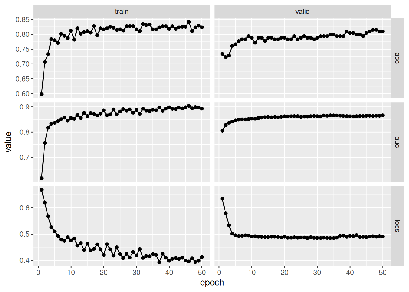
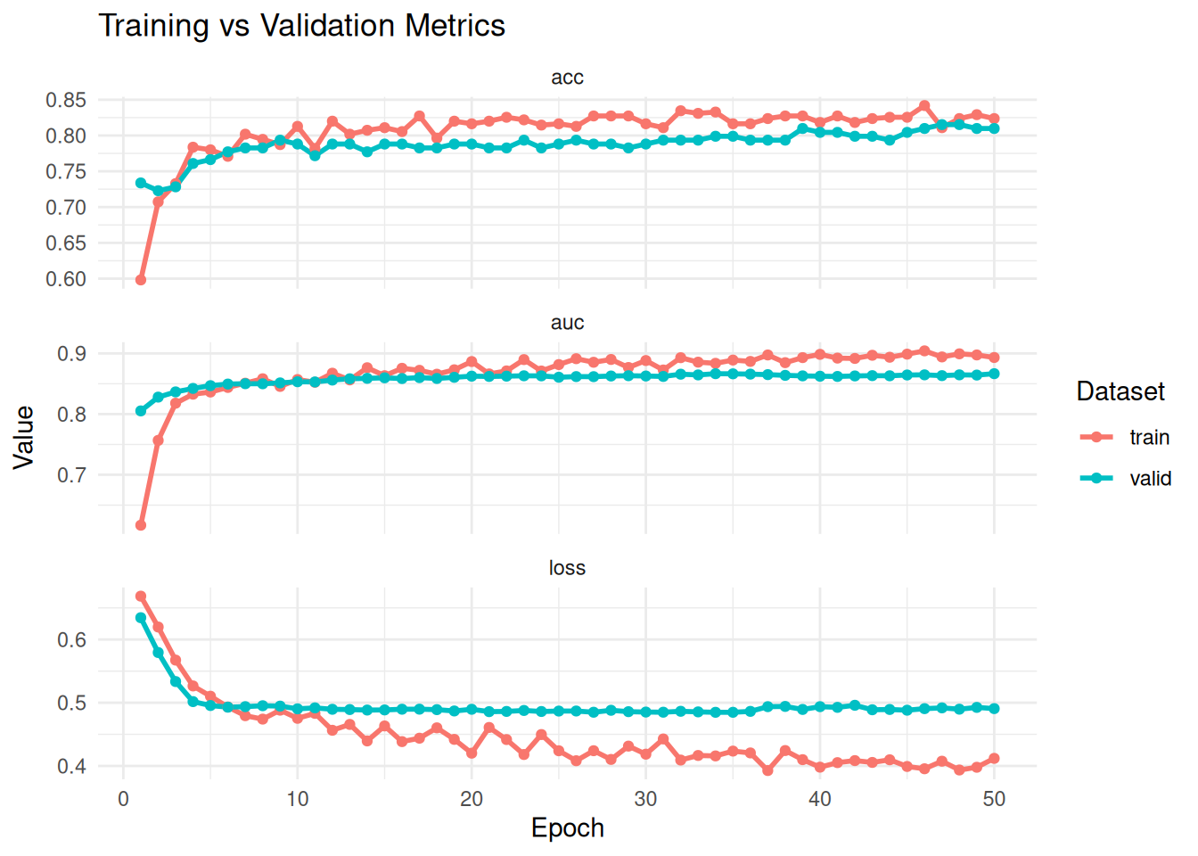
Better plot
hist <- get_metrics(fitted)

hist %>%
ggplot(aes(x = epoch, y = value, color = set)) +
geom_line(linewidth = 1) + # Draw lines
geom_point(size = 1.5) + # Add points for clarity
facet_wrap(~ metric, scales = "free_y", ncol = 1) + # Stack metrics vertically
theme_minimal() +
labs(
    title = "Training vs Validation Metrics",
    y = "Value",
    x = "Epoch",
    color = "Dataset"
)
Re-fit the model
Fit
fitted2 <-
net %>%
setup(
    loss = nn_bce_loss(),
    optimizer = optim_adam,
    metrics = list(
        luz_metric_binary_accuracy(),
        luz_metric_binary_auroc() )
) %>%
set_hparams(d_in = d_in) %>%
fit(
    train_dl,
    epoch = 5,
    valid_data = val_dl
)
Predict testing set
y_pred <- fitted2 %>% predict(test_dl)

dat_pred <-
y_pred %>%
as_array() %>%
as_tibble(.name_repair = "unique") %>%
 rename(prob = 1) %>%
mutate(
    pred = factor(ifelse(prob > 0.5, 1, 0)),
    true = factor(heart_test$HeartDisease)
    )
New names:
• `` -> `...1`dat_pred# A tibble: 184 × 3
prob pred true
<dbl> <fct> <fct>
1 0.327 0 1
2 0.411 0 0
3 0.775 1 1
4 0.615 1 1
5 0.303 0 0
6 0.258 0 0
7 0.289 0 0
8 0.535 1 0
9 0.686 1 0
10 0.170 0 0
# ℹ 174 more rowsEvaluate
fitted %>% evaluate(test_dl) # Less accurateA `luz_module_evaluation`
── Results ─────────────────────────────────────────────────────────────────────
loss: 0.379
acc: 0.837
auc: 0.9039Confusion matrix
dat_pred %>%
conf_mat(true, pred) %>%
autoplot("heatmap")
Accuracy
dat_pred %>%
accuracy(truth = true, estimate = pred)
# A tibble: 1 × 3
.metric .estimator .estimate
<chr> <chr> <dbl>
1 accuracy binary 0.837Plot ROC
dat_pred %>%
roc_curve(true, prob, event_level = "second") %>%
autoplot()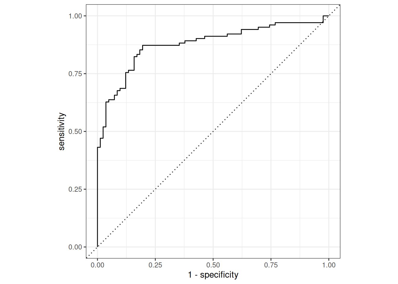
# ROC-AUC
dat_pred %>%
roc_auc(true, prob, event_level = "second")
# A tibble: 1 × 3
.metric .estimator .estimate
<chr> <chr> <dbl>
1 roc_auc binary 0.878