9  Data exploration

“Data is like garbage. You’d better know what you are going to do with it before you collect it.”

– Mark Twain

Data exploration, as the name suggests involves the process of exploring the data to understand its structures, identifying underlying patterns, and discovering its characteristics. This process is the first stage in analysing the data and gaining insight from it. Doing data analysis without data exploration is akin to going to war without a proper strategy.

R provides numerous functions and packages that can help to explore the data efficiently and systematically. Thus, this chapter intends to introduce those functions and packages to readers adequately and further equip the readers to do any data analysis.

9.1 Missing data

Missing data are recognised as NA in R. Let’s use airquality data, a built-in dataset in R to see how R recognised missing values.

# Data with missing data
data("airquality")

By using summary(), we can see that the first two columns have missing values, recognised as NA.

summary(airquality)

     Ozone           Solar.R           Wind             Temp      
 Min.   :  1.00   Min.   :  7.0   Min.   : 1.700   Min.   :56.00  
 1st Qu.: 18.00   1st Qu.:115.8   1st Qu.: 7.400   1st Qu.:72.00  
 Median : 31.50   Median :205.0   Median : 9.700   Median :79.00  
 Mean   : 42.13   Mean   :185.9   Mean   : 9.958   Mean   :77.88  
 3rd Qu.: 63.25   3rd Qu.:258.8   3rd Qu.:11.500   3rd Qu.:85.00  
 Max.   :168.00   Max.   :334.0   Max.   :20.700   Max.   :97.00  
 NA's   :37       NA's   :7                                       
     Month            Day      
 Min.   :5.000   Min.   : 1.0  
 1st Qu.:6.000   1st Qu.: 8.0  
 Median :7.000   Median :16.0  
 Mean   :6.993   Mean   :15.8  
 3rd Qu.:8.000   3rd Qu.:23.0  
 Max.   :9.000   Max.   :31.0  
                               

Another function to give a quick answer to whether we have available data or not is anyNA().

anyNA(airquality)

[1] TRUE

To get the count of missing values, we can use is.na():

is.na(airquality) |> table()

FALSE  TRUE 
  874    44 

TRUE is 44, which means that we have 44 missing values across individual cells in our dataset. To drop the missing values, we can use complete.cases():

# Make an index
na_index <- complete.cases(airquality)

# Apply the index to drop the NA's
airquality_noNA <- airquality[na_index, ]

Alternatively, it is easier to use na.omit():

airquality_noNA2 <- na.omit(airquality)

Both, complete.cases() and na.omit() return an identical output.

# Drop NA's using complete.cases()
dim(airquality_noNA)

[1] 111   6

# Drop NA's using na.omit()
dim(airquality_noNA2)

[1] 111   6

We may want to explore the data with missing values. Thus, we can use complete.cases() plus ! in our codes to isolate the data with missing values.

# Make an index
na_index <- complete.cases(airquality)

# Apply the index to drop the NA's
airquality_NA_only <- airquality[!na_index, ]

# Data with missing values
dim(airquality_NA_only)

[1] 42  6

Notice that the airquality_NA_only returns 44 rows of data with missing values, while using is.na() earlier we get 44 missing values. airquality_NA_only returns rows of data with missing values. The missing values may exist in more than a single column in the dataset. The is.na() function counts all the missing values regardless of the position.

9.2 Outliers

An outlier is a data point that lies significantly outside the range of most other observations in a dataset. It is an extreme value, either unusually high or low, that differs markedly from other data points. Outliers can occur due to variability in the data, errors in measurement, or experimental anomalies.

Since outliers may not be representative of the data and may distort statistical measures such as mean and standard deviation, it is important to identify them early during the data exploration stage.

There are two methods to identify outliers:

1. Interquartile range (IQR) or box plot method:

   The IQR method identifies outliers as data points lying below Q1 − 1.5 × IQR or above Q3 + 1.5 × IQR , where Q1 and Q3 are the first and third quartiles, respectively. This is the method that applies in the boxplot.

   Let’s use airquality_noNA data to demonstrate:

   out_bp <- boxplot(airquality_noNA$Wind, main = "Outliers in the wind column")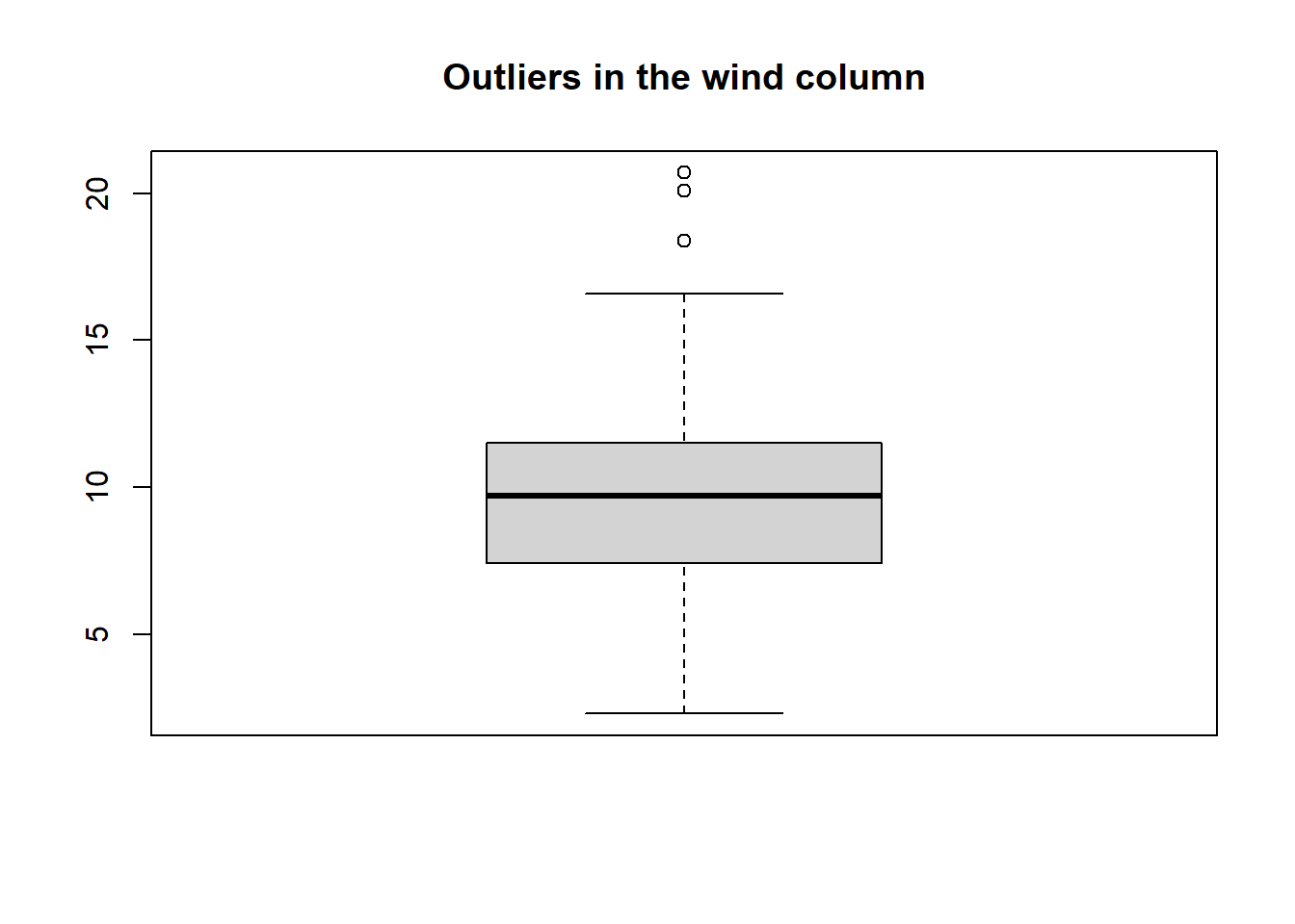

   

   To access the values of the outliers:

   out_bp$out

   [1] 20.1 18.4 20.7

   To see the rows with the outliers:

   airquality_noNA |> 
     dplyr::filter(Wind == c(20.1, 18.4, 20.7))

     Ozone Solar.R Wind Temp Month Day
   1     8      19 20.1   61     5   9
   2     6      78 18.4   57     5  18
   3    37     284 20.7   72     6  17

2. Z-score method:

   This method standardizes data and identifies outliers as those with a z-score greater than a threshold (commonly 3 or -3). The z-score (also called a standard score) is a statistical measure that indicates how many standard deviations a data point is from the mean of the dataset.

   Basically, the z-score is a distribution which reflects our dataset and it shows how far each value is from the average. So, in this context, outliers are the values that are significantly far from the average.

   Now, let’s focus on understanding how we can detect the outliers using this method.

   # Create z-score for the data
   z_scores <- scale(airquality_noNA$Wind)
   
   # How many outliers
   table(abs(z_scores) > 3)

   
   FALSE  TRUE 
     110     1 

   TRUE is 1, which means that we have a single outlier in our data. Let’s see which value is the outlier.

   airquality_noNA$Wind[abs(z_scores) > 3]

   [1] 20.7

   To see the row with the outlier:

   airquality_noNA |> 
     dplyr::filter(Wind == 20.7)

     Ozone Solar.R Wind Temp Month Day
   1    37     284 20.7   72     6  17

There is a useful package where we can check for outliers more effficently, which is the perfomance package. One of the benefits of using this package compared to the base R approach that we covered earlier is that this package can easily check the outliers for the whole dataset.

First, let us install the package.

install.packages("performance")

Now, let us load the package.

To check the outliers using the IQR method:

iqr_outliers <- check_outliers(airquality_noNA, method = "iqr", threshold = 2)
iqr_outliers

3 outliers detected: cases 7, 30, 77.
- Based on the following method and threshold: iqr (2).
- For variables: Ozone, Solar.R, Wind, Temp, Month, Day.

-----------------------------------------------------------------------------
Outliers per variable (iqr): 

$Ozone
   Row Distance_IQR
77  77     1.454545

$Wind
   Row Distance_IQR
7    7     1.298780
30  30     1.371951

method specify the method that we want to use to detect the outliers and threshold specify the threshold for each method. In IQR method, the outliers are determined using these formula:

\(outliers < Q1 - (IQR * 1.5)\) or \(outliers > Q3 + (IQR * 1.5)\)

The value of 1.5 is proposed by John Tukey, the famous statistician who founded this method. However, the performance package uses 2 as the threshold by default. The IQR method from the base R that we learnt earlier used the threshold of 1.5.

If we want to extract the outliers:

# This will extract the row positions of outliers 
iqr_outliers_points <- which(iqr_outliers)

# Extract from the data
airquality_noNA %>% 
  slice(iqr_outliers_points)

  Ozone Solar.R Wind Temp Month Day
1     8      19 20.1   61     5   9
2    37     284 20.7   72     6  17
3   168     238  3.4   81     8  25

Next, let us see the z-score method using the performance package.

zs_outliers <- check_outliers(airquality_noNA, method = "zscore", threshold = 3)
zs_outliers

2 outliers detected: cases 30, 77.
- Based on the following method and threshold: zscore (3).
- For variables: Ozone, Solar.R, Wind, Temp, Month, Day.

-----------------------------------------------------------------------------
Outliers per variable (zscore): 

$Ozone
   Row Distance_Zscore
77  77        3.783538

$Wind
   Row Distance_Zscore
30  30        3.024516

The arguments are similar since we are using the same function. For the z-score method, we often look at the threshold to decide how extreme a value must be to be labeled an outlier.

• A threshold of 3.291 (the default in performance package for this method) is a conservative choice. It identifies only the most extreme values (roughly the top 0.1% of a normal distribution).
• A threshold of 3 is more sensitive. It will identify more points as outliers (roughly the top 0.3% of extreme values).

Additionally, we can get the outliers by using the same function as previously:

# This will extract the row positions of outliers 
zs_outliers_points <- which(zs_outliers)

# Extract from the data
airquality_noNA %>% 
  slice(zs_outliers_points)

  Ozone Solar.R Wind Temp Month Day
1    37     284 20.7   72     6  17
2   168     238  3.4   81     8  25

There are other advanced methods to detect outliers in the performance package (you can read more on the method argument by typing ?check_outliers() in the console). However, the basics to understand those methods are beyond the scope of this book.

9.3 Useful packages

In this section, we going to see several useful R packages to explore the data. We are only going to cover the main functions of each package.

9.3.1 skimr

The skimr package provides various helpful functions to do data exploration. Firstly, we need to install skimr, and then load the packages. We going to use the dplyr package together with the skimr package.

# Install the package
install.packages("skimr")

# Load the necessary packages
library(skimr)
library(dplyr)

To explore the whole dataset, we can use skim.

# Let's use the iris dataset
data("iris")

# Use skim
skim(iris)

Data summary

Name	iris
Number of rows	150
Number of columns	5
_______________________
Column type frequency:
factor	1
numeric	4
________________________
Group variables	None

Variable type: factor

skim_variable	n_missing	complete_rate	ordered	n_unique	top_counts
Species	0	1	FALSE	3	set: 50, ver: 50, vir: 50

Variable type: numeric

skim_variable	n_missing	complete_rate	mean	sd	p0	p25	p50	p75	p100	hist
Sepal.Length	0	1	5.84	0.83	4.3	5.1	5.80	6.4	7.9	▆▇▇▅▂
Sepal.Width	0	1	3.06	0.44	2.0	2.8	3.00	3.3	4.4	▁▆▇▂▁
Petal.Length	0	1	3.76	1.77	1.0	1.6	4.35	5.1	6.9	▇▁▆▇▂
Petal.Width	0	1	1.20	0.76	0.1	0.3	1.30	1.8	2.5	▇▁▇▅▃

The skim function will return the basic statistics for our data including the information on the missing values (n_missing and complete_rate) and a histogram for the numerical variables. Additionally, we can get the basic statistics based on a certain group. For example, here we use group_by(), then, we apply skim().

iris %>% 
  group_by(Species) %>% 
  skim()

Data summary

Name	Piped data
Number of rows	150
Number of columns	5
_______________________
Column type frequency:
numeric	4
________________________
Group variables	Species

Variable type: numeric

skim_variable	Species	n_missing	complete_rate	mean	sd	p0	p25	p50	p75	p100	hist
Sepal.Length	setosa	0	1	5.01	0.35	4.3	4.80	5.00	5.20	5.8	▃▃▇▅▁
Sepal.Length	versicolor	0	1	5.94	0.52	4.9	5.60	5.90	6.30	7.0	▂▇▆▃▃
Sepal.Length	virginica	0	1	6.59	0.64	4.9	6.23	6.50	6.90	7.9	▁▃▇▃▂
Sepal.Width	setosa	0	1	3.43	0.38	2.3	3.20	3.40	3.68	4.4	▁▃▇▅▂
Sepal.Width	versicolor	0	1	2.77	0.31	2.0	2.52	2.80	3.00	3.4	▁▅▆▇▂
Sepal.Width	virginica	0	1	2.97	0.32	2.2	2.80	3.00	3.18	3.8	▂▆▇▅▁
Petal.Length	setosa	0	1	1.46	0.17	1.0	1.40	1.50	1.58	1.9	▁▃▇▃▁
Petal.Length	versicolor	0	1	4.26	0.47	3.0	4.00	4.35	4.60	5.1	▂▂▇▇▆
Petal.Length	virginica	0	1	5.55	0.55	4.5	5.10	5.55	5.88	6.9	▃▇▇▃▂
Petal.Width	setosa	0	1	0.25	0.11	0.1	0.20	0.20	0.30	0.6	▇▂▂▁▁
Petal.Width	versicolor	0	1	1.33	0.20	1.0	1.20	1.30	1.50	1.8	▅▇▃▆▁
Petal.Width	virginica	0	1	2.03	0.27	1.4	1.80	2.00	2.30	2.5	▂▇▆▅▇

Readers interested in learning more about the skimr package can explore its comprehensive documentation for more details and examples.

9.3.2 naniar

naniar package provides tidy ways to summarise, visualise, and manipulate missing data. First, let’s install and load the necessary packages.

# Install the package
install.packages("naniar")

# Load the necessary packages
library(naniar)
library(dplyr)

Let’s use the oceanbuoys data, a dataset from the naniar package. First, let’s summarise the missing data according to a variable. Further detail on the dataset can be found by running ?oceanbuoys in the Console.

# Load the data
data("oceanbuoys")

# Missing values summary based on variables
miss_var_summary(oceanbuoys)

# A tibble: 8 × 3
  variable   n_miss pct_miss
  <chr>       <int>    <num>
1 humidity       93   12.6  
2 air_temp_c     81   11.0  
3 sea_temp_c      3    0.408
4 year            0    0    
5 latitude        0    0    
6 longitude       0    0    
7 wind_ew         0    0    
8 wind_ns         0    0    

n_miss is the number of missing values and pct_miss is the percentage of missing values. We can further group the missing values according to a certain variable.

oceanbuoys %>% 
  group_by(year) %>% 
  miss_var_summary()

# A tibble: 14 × 4
# Groups:   year [2]
    year variable   n_miss pct_miss
   <dbl> <chr>       <int>    <num>
 1  1997 air_temp_c     77   20.9  
 2  1997 latitude        0    0    
 3  1997 longitude       0    0    
 4  1997 sea_temp_c      0    0    
 5  1997 humidity        0    0    
 6  1997 wind_ew         0    0    
 7  1997 wind_ns         0    0    
 8  1993 humidity       93   25.3  
 9  1993 air_temp_c      4    1.09 
10  1993 sea_temp_c      3    0.815
11  1993 latitude        0    0    
12  1993 longitude       0    0    
13  1993 wind_ew         0    0    
14  1993 wind_ns         0    0    

naniar also provides a visual summary for missing values.

gg_miss_var(oceanbuoys)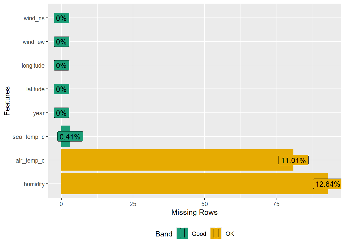

We can further group by a variable using the facet argument.

gg_miss_var(oceanbuoys, facet = year)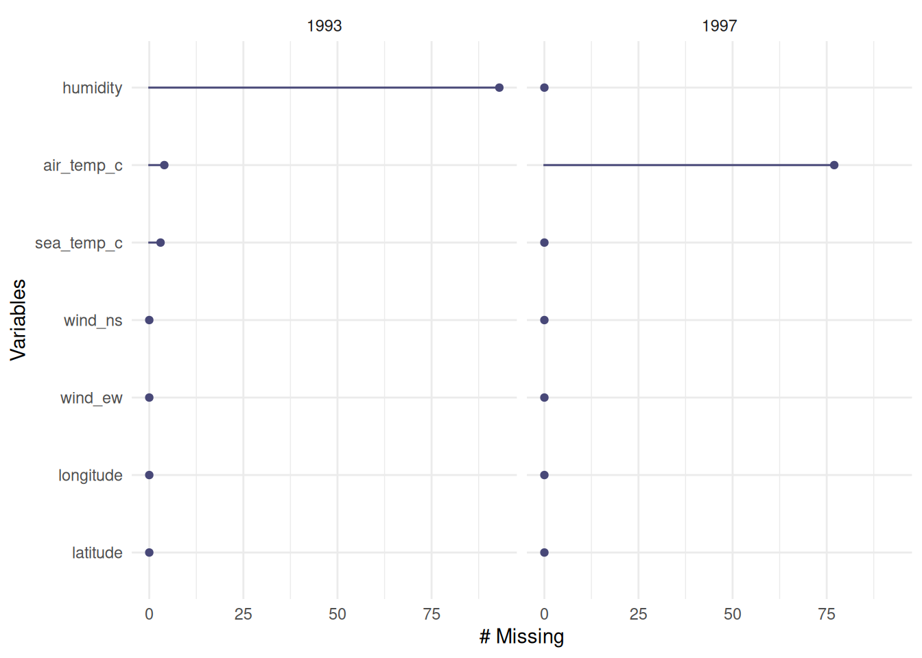

The content we just covered provides only a glimpse of the powerful features and capabilities of the naniar package. For a deeper understanding and comprehensive insights, readers are encouraged to explore the naniar documentation website.

9.3.3 DataExplorer

DataExplorer provides various helpful functions for data exploration. First, let’s install and load the necessary packages.

# Install package
install.packages("DataExplorer")

# Load the necessary packages
library(DataExplorer)
library(dplyr)

Let’s use oceanbuoys data from the naniar package previously.

# Load the data 
data("oceanbuoys", package = "naniar")

DataExplorer provides a general function to explore the data.

plot_intro(oceanbuoys)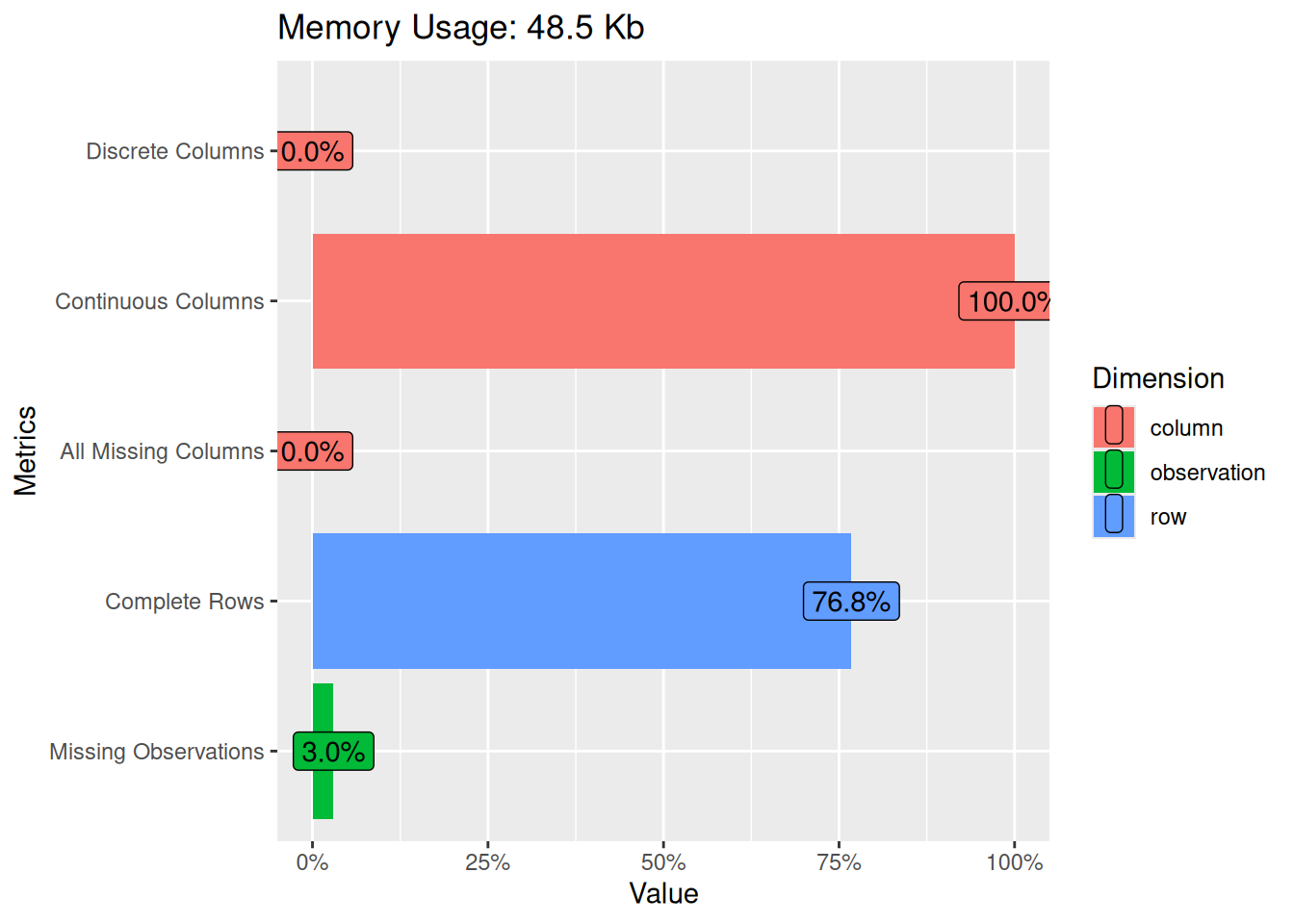

From the plot, we understand that our data consists of all continuous (numeric) columns and no discrete (categorical) columns. No missing columns but we have 3% missing observations.

To investigate the missing observations, we can use plot_missing():

plot_missing(oceanbuoys)

Warning: `aes_string()` was deprecated in ggplot2 3.0.0.
ℹ Please use tidy evaluation idioms with `aes()`.
ℹ See also `vignette("ggplot2-in-packages")` for more information.
ℹ The deprecated feature was likely used in the DataExplorer package.
  Please report the issue at
  <https://github.com/boxuancui/DataExplorer/issues>.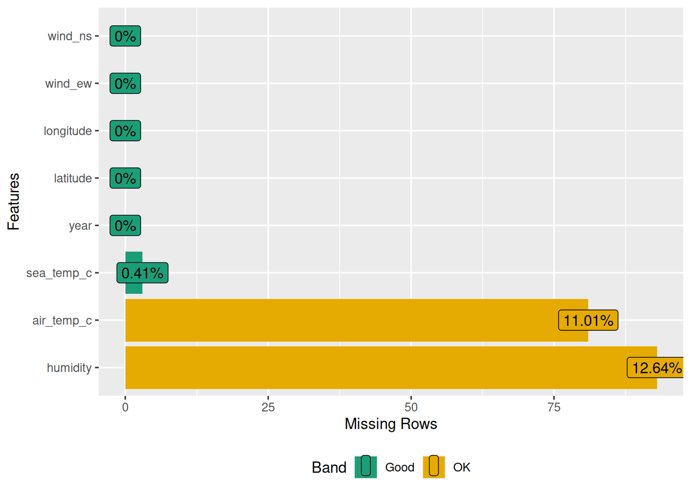

Alternatively, we can get a summary instead of a plot.

profile_missing(oceanbuoys)

# A tibble: 8 × 3
  feature    num_missing pct_missing
  <fct>            <int>       <dbl>
1 year                 0     0      
2 latitude             0     0      
3 longitude            0     0      
4 sea_temp_c           3     0.00408
5 air_temp_c          81     0.110  
6 humidity            93     0.126  
7 wind_ew              0     0      
8 wind_ns              0     0      

Additionally, DataExplorer provides a function to plot a correlation matrix. Correlation is a measure of association between two numerical variables. It ranges between -1 and 1. Values close to 1 indicate a high positive correlation between the two variables, while values close to -1 indicate a high negative correlation between the two numerical variables. Values close to 0 indicate a low correlation between the two values.

oceanbuoys %>% 
  na.omit() %>% 
  plot_correlation()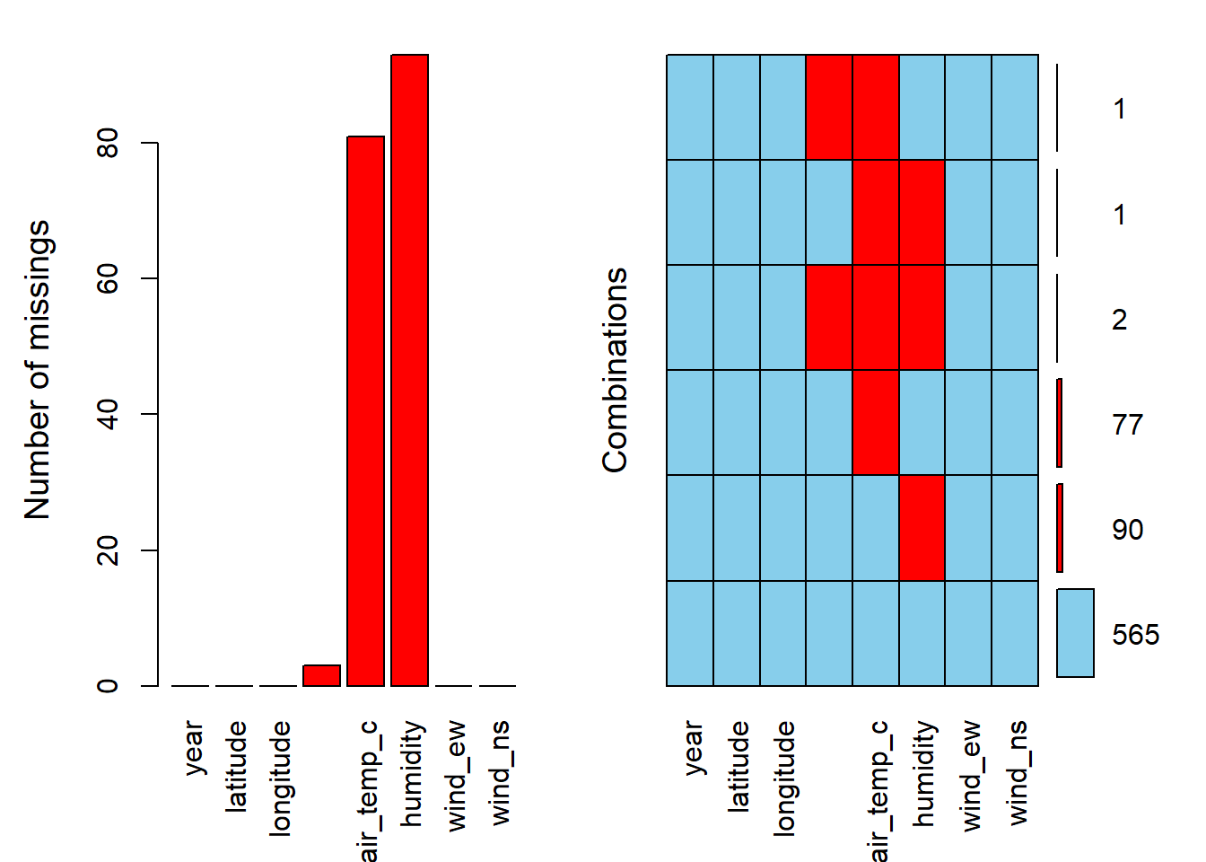

To do a correlation or in this case correlation plot, the variables should be numerical and have no missing values (hence, the use of na.omit() in the code). If for example, we want to apply this function to the iris dataset, in which we know that one of the variables is categorical, we need to exclude the variable first.

iris %>% 
  select(-Species) %>% 
  plot_correlation()

Alternatively, the more efficient code to exclude the non-numerical variable is using the select_if().

iris %>% 
  select_if(is.numeric) %>% 
  plot_correlation()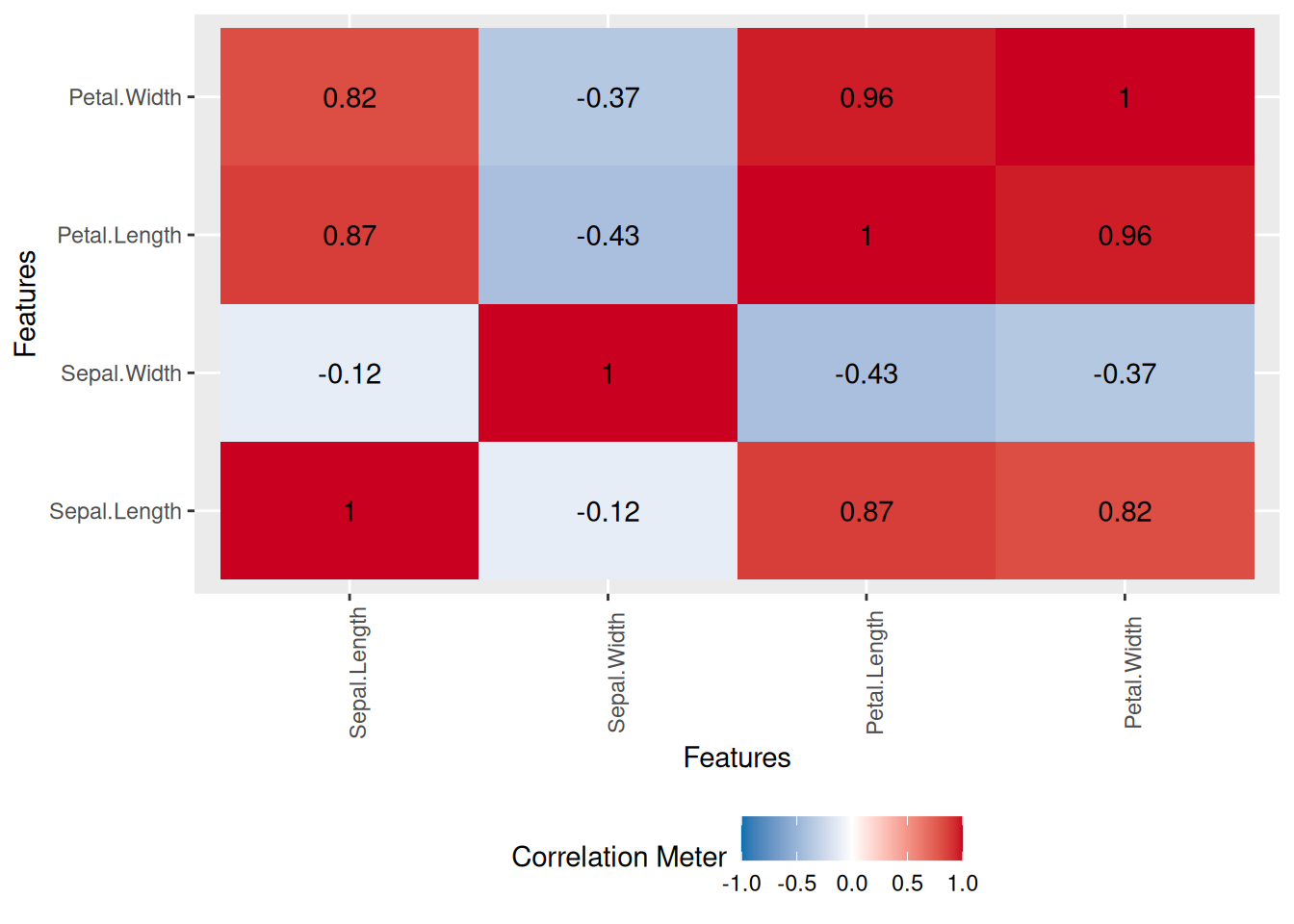

DataExplorer provides more useful functions, which can not be extensively covered in this section. Interested readers can further study its documentation for more.

9.3.4 VIM

The VIM package contains tools for the visualisation of missing and/or imputed values. Imputation of the missing values is beyond the scope of this book. However, we going to see how functions from the VIM package can be utilised to explore the pattern of missingness.

First, make sure to install the VIM package and load the necessary packages.

# Install package
install.packages("VIM")

# Load the necessary packages
library(VIM)
library(dplyr)

Let’s use oceanbuoys data from the naniar package previously.

# Load the data 
data("oceanbuoys", package = "naniar")

The aggr() function will plot our data and visualise the pattern of missing values. numbers = TRUE and prop = FALSE to make sure the number missing values in a number not a proportion.

aggr(oceanbuoys, numbers = TRUE, prop = FALSE)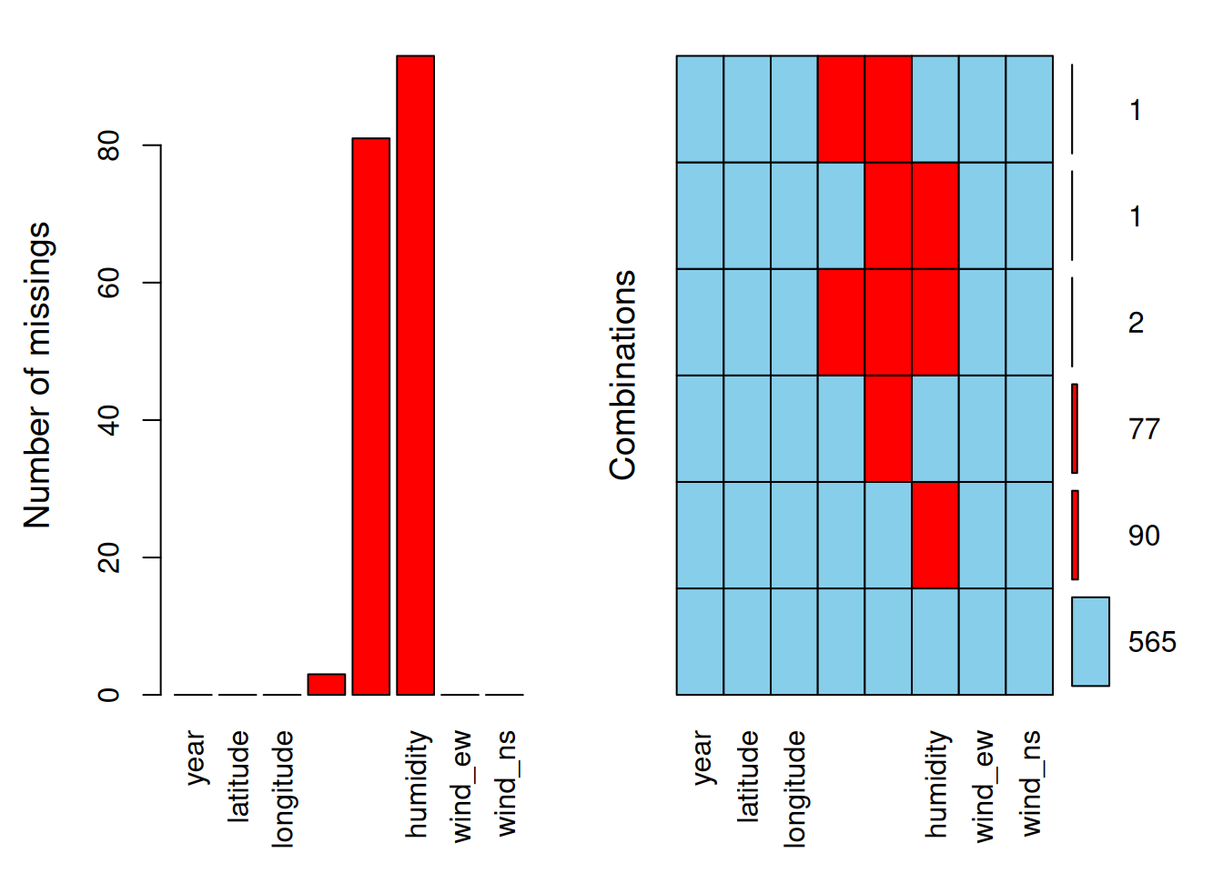

The red colour represents the missing values, and the blue colour represents the observed values. The first plot on the left presents the proportion of missing values according to variables. The second plot on the right presents the combination of missing values. Notice that if we have too many variables, the variable names will not be fully displayed. For example in the second plot, for a combination of sea_temp_c, air_temp_c, and humidity, we have 2 values missing.

The aggr() function is suitable to be utilised when we have a small to intermediate number of variables. For data with a large number of variables, matrixplot() may be more appropriate.

matrixplot(oceanbuoys)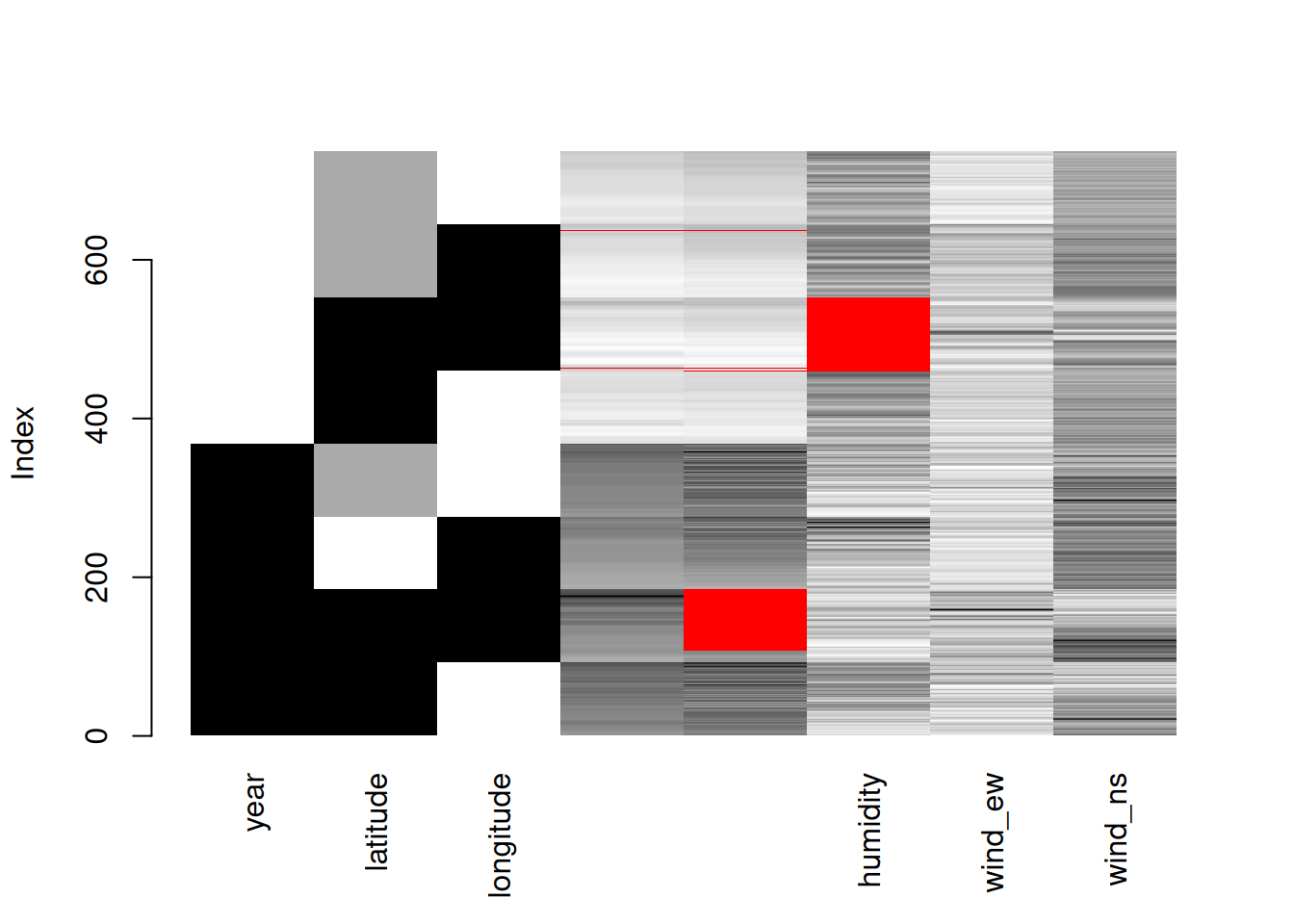

matrixplot() scales the data into 0 (white) and 1 (black). The higher values will become close to 1, and the lower values will become close to 0. The red colour represents the missing values.

The VIM package contains more useful functions, however, the majority of them are for exploring the imputation methods and values. Interested readers can further study its documentation for more details.

9.3.5 dlookr

The dlookr package provides various helpful functions especially related to outliers. First, we need to install the dlookr package and load the necessary packages.

# Install package
install.packages("dlookr")

# Load the packages
library(dlookr)
library(dplyr)

Let’s use the Carseats dataset, a dataset from dlookr package. The diagnose_numeric() function from the dlookr package is particularly useful for diagnosing numeric variables.

# Load the data
data("Carseats")

# Diagnose function
diagnose_numeric(Carseats)

    variables min     Q1       mean median     Q3    max zero minus outlier
1       Sales   0   5.39   7.496325   7.49   9.32  16.27    1     0       2
2   CompPrice  77 115.00 124.975000 125.00 135.00 175.00    0     0       2
3      Income  21  42.75  68.657500  69.00  91.00 120.00    0     0       0
4 Advertising   0   0.00   6.635000   5.00  12.00  29.00  144     0       0
5  Population  10 139.00 264.840000 272.00 398.50 509.00    0     0       0
6       Price  24 100.00 115.795000 117.00 131.00 191.00    0     0       5
7         Age  25  39.75  53.322500  54.50  66.00  80.00    0     0       0
8   Education  10  12.00  13.900000  14.00  16.00  18.00    0     0       0

Among its results, it provides the following insights:

• zero: the number of zero values in the data.
• minus: the count of negative values.
• outlier: the number of potential outliers detected in the dataset.

Additionally, we have diagnose_category() which summarises categorical variables. This function returns several outputs:

• levels: level for each categorical variable.
• N: number of observations.
• freq: number of observations at the levels.
• ratio: percentage of observations at the levels
• rank: rank of occupancy ratio of levels

diagnose_category(Carseats)

  variables levels   N freq ratio rank
1 ShelveLoc Medium 400  219 54.75    1
2 ShelveLoc    Bad 400   96 24.00    2
3 ShelveLoc   Good 400   85 21.25    3
4     Urban    Yes 400  282 70.50    1
5     Urban     No 400  118 29.50    2
6        US    Yes 400  258 64.50    1
7        US     No 400  142 35.50    2

We can further explore the outliers identified by diagnose_numeric() using diagnose_outlier().

diagnose_outlier(Carseats)

    variables outliers_cnt outliers_ratio outliers_mean  with_mean without_mean
1       Sales            2           0.50         15.95   7.496325     7.453844
2   CompPrice            2           0.50        126.00 124.975000   124.969849
3      Income            0           0.00           NaN  68.657500    68.657500
4 Advertising            0           0.00           NaN   6.635000     6.635000
5  Population            0           0.00           NaN 264.840000   264.840000
6       Price            5           1.25        100.40 115.795000   115.989873
7         Age            0           0.00           NaN  53.322500    53.322500
8   Education            0           0.00           NaN  13.900000    13.900000

This function returns:

• outliers_cnt: number of outliers.
• outliers_ratio: percent of outliers.
• outliers_mean: mean of outliers.
• with_mean: mean of values with outliers.
• without_mean: mean of values of without outliers.

In fact, we can further simplify the result using the filter() from the dplyr package.

diagnose_outlier(Carseats) %>% 
  filter(outliers_cnt > 0)

  variables outliers_cnt outliers_ratio outliers_mean  with_mean without_mean
1     Sales            2           0.50         15.95   7.496325     7.453844
2 CompPrice            2           0.50        126.00 124.975000   124.969849
3     Price            5           1.25        100.40 115.795000   115.989873

Furthermore, dlookr provides another useful function to visualise the outliers. However, for this example, we going to select a single variable.

Carseats %>% 
  select(Sales) %>% 
  plot_outlier()

Warning: The `size` argument of `element_line()` is deprecated as of ggplot2 3.4.0.
ℹ Please use the `linewidth` argument instead.
ℹ The deprecated feature was likely used in the dlookr package.
  Please report the issue at <https://github.com/choonghyunryu/dlookr/issues>.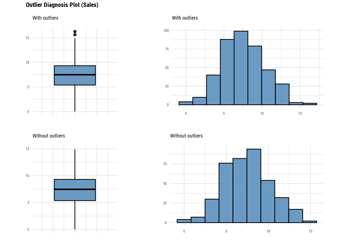

This function returns a boxplot and histogram for values with and without outliers. Thus, we can see how much the outliers in the variables change the distribution of the data. dlookr actually provides more functions than the ones we covered in this section. Readers are suggested to go through its documentation to further learn this package.

9.4 Chapter summary

In this chapter, we have covered how missing data and outliers were identified in R using base R functions. Moreover, we have covered several useful functions from five R packages:

1. skimr
2. naniar
3. DataExplorer
4. VIM
5. dlookr

skimr provides general functions for data exploration (Waring et al. 2024). naniar, DataExplorer, and VIM provide additional functions to explore and investigate missing data (Tierney and Cook 2023; Cui 2024; Kowarik and Templ 2016). Lastly, dlookr provides more functions for investigating outliers in the dataset (Ryu 2024).

While this chapter highlights the capabilities of these five packages, it is important to note that R offers many additional packages that can further enhance your analysis. Readers are encouraged to explore beyond these tools to find packages best suited to their specific needs.

9.5 Revision

1. Why is data exploration considered a crucial first step in data analysis, and what are some R functions and packages that can help in this process?

2. Write an R code to check for missing values in each column of the riskfactors dataset, a dataset from the naniar package. Then, count how many NA values exist in total.

   # Load the data
   data("riskfactors", package = "naniar")

3. Using the riskfactors dataset from question 2, write R code to remove all missing values in the dataset and determine how many rows are left.

4. Besides dropping the missing values, what are the possible solutions to missing values?

5. What are the possible solutions for outliers?

6. What are the pros and cons of dropping:

   1. Missing values
   2. Outliers

7. Name three packages for data exploration besides the five packages covered in this chapter.

Cui, Boxuan. 2024. DataExplorer: Automate Data Exploration and Treatment. http://boxuancui.github.io/DataExplorer/.

Kowarik, Alexander, and Matthias Templ. 2016. “Imputation with the r Package VIM.” Journal of Statistical Software 74 (7): 1–16. https://doi.org/10.18637/jss.v074.i07.

Ryu, Choonghyun. 2024. Dlookr: Tools for Data Diagnosis, Exploration, Transformation. https://CRAN.R-project.org/package=dlookr.

Tierney, Nicholas, and Dianne Cook. 2023. “Expanding Tidy Data Principles to Facilitate Missing Data Exploration, Visualization and Assessment of Imputations.” Journal of Statistical Software 105 (7): 1–31. https://doi.org/10.18637/jss.v105.i07.

Waring, Elin, Michael Quinn, Amelia McNamara, Eduardo Arino de la Rubia, Hao Zhu, and Shannon Ellis. 2024. Skimr: Compact and Flexible Summaries of Data. https://docs.ropensci.org/skimr/.